
- Home
- Tutorials
- Data Science
- Linear Algebra & Matrices
Linear Algebra for Data Science: Vectors, Matrices & Geometric Intuition
If data is the fuel of modern artificial intelligence, Linear Algebra is the mathematical engine. In this class, we build intuitive geometric foundations of vector spaces, matrix transformations, norms, dot products, and analytical linear regression derivations.
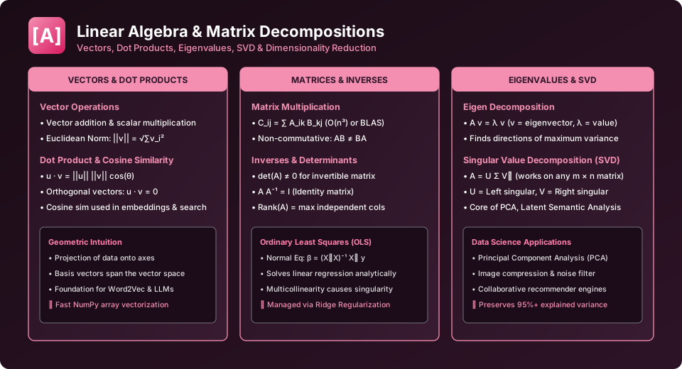
Figure 7.1: Geometric Vectors, Dot Products, Matrix Inverses & Ordinary Least Squares (OLS).
1. Vectors as Points in Multi-Dimensional Space
In data science, a single customer profile with features [Age: 28, Income: 65000, Purchases: 14] is represented as a 3-dimensional vector in \(\mathbb{R}^3\):
\[ \mathbf{v} = \begin{bmatrix} 28 \\ 65000 \\ 14 \end{bmatrix} \]Vector Norms (Length and Distance)
- \(L_2\) Euclidean Norm (Length): Standard straight-line distance from the origin: \[ ||\mathbf{v}||_2 = \sqrt{\sum_{i=1}^{n} v_i^2} \] This norm is the core loss metric of Ordinary Least Squares regression and Ridge regularization.
- \(L_1\) Manhattan Norm: Sum of absolute coordinate distances: \[ ||\mathbf{v}||_1 = \sum_{i=1}^{n} |v_i| \] Powers Lasso regularization, driving uninformative feature weights to exact zero.
2. The Dot Product and Cosine Similarity
The algebraic dot product sums the element-wise products of two vectors:
\[ \mathbf{u} \cdot \mathbf{v} = \sum_{i=1}^{n} u_i v_i = ||\mathbf{u}|| \, ||\mathbf{v}|| \cos(\theta) \]Rearranging for \(\cos(\theta)\) yields Cosine Similarity — the global standard metric used in modern AI vector databases (PostgreSQL pgvector, Pinecone, Chroma):
\[ \text{Cosine Similarity}(\mathbf{u}, \mathbf{v}) = \frac{\mathbf{u} \cdot \mathbf{v}}{||\mathbf{u}|| \, ||\mathbf{v}||} \]3. The Analytical OLS Solution (Normal Equation)
In simple and multiple linear regression, the goal is to find weight vector \(\mathbf{\beta}\) that minimizes the sum of squared prediction residuals: \(L(\mathbf{\beta}) = ||\mathbf{y} - \mathbf{X}\mathbf{\beta}||_2^2\). Taking the matrix derivative and setting it to zero produces the famous Normal Equation:
\[ \mathbf{\beta} = (\mathbf{X}^T \mathbf{X})^{-1} \mathbf{X}^T \mathbf{y} \]NumPy Hands-on: Vector Operations & Normal Equation
import numpy as np

# Define two customer embedding vectors
u = np.array([0.24, 0.88, -0.45])
v = np.array([0.31, 0.82, -0.40])

# Compute Dot Product & Cosine Similarity
dot_prod = np.dot(u, v)
cos_sim = dot_prod / (np.linalg.norm(u) * np.linalg.norm(v))
print(f"Dot Product:        {dot_prod:.4f}")
print(f"Cosine Similarity:  {cos_sim:.4f} (Very high directional alignment)")

# Solving Linear Regression via OLS Normal Equation
X = np.array([[1, 2], [1, 3], [1, 4], [1, 5]])  # Bias column + feature
y = np.array([5.1, 7.0, 9.2, 10.9])

beta = np.linalg.inv(X.T @ X) @ X.T @ y
print(f"Intercept: {beta[0]:.3f}, Slope: {beta[1]:.3f}")
University Viva & Exam Checklist
Explain why \(\mathbf{X}^T\mathbf{X}\) is always a symmetric square matrix. What happens when two feature columns in \(\mathbf{X}\) are perfectly correlated? (Answer: The determinant of \(\mathbf{X}^T\mathbf{X}\) becomes 0, matrix inversion fails, and regularized Ridge regression must be used).
Frequently Asked Questions (FAQ) - Student & Interview Review
Q1. Why is Linear Algebra fundamental to Data Science?
Q2. What does the dot product geometrically represent?
Q3. How does cosine similarity differ from Euclidean distance?
Q4. What is matrix rank and why does it matter in regression?
Q5. How does NumPy accelerate linear algebra operations?
Explore Related Data Science Tutorials & Next Steps
Broaden your statistical analysis, Python data wrangling, and production engineering expertise:
Understand spectral decomposition, principal axes, and singular value decomposition.
Derive gradients and loss function Jacobians for optimization.
Write lightning-fast linear algebra routines using Python's NumPy library.
Store and index dense vector embeddings for semantic similarity search.


You may also like this!
© Veewom.com. | Managed by PinePL
