Convolutional Neural Networks (CNN) for Computer Vision

If we feed a 1000 × 1000 RGB image (3,000,000 values) into a standard Multi-Layer Perceptron (MLP) with 1,000 hidden neurons, the first layer alone requires 3 billion weights! Furthermore, flattening 2D images into 1D vectors destroys all spatial geometric proximity. Convolutional Neural Networks (CNNs) solve this through Local Receptive Fields, Shared Weights, and Spatial Invariance.

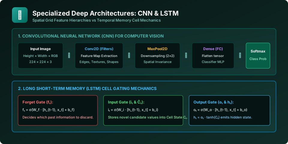
Figure 33.1: The Convolutional Neural Network (CNN) Feature Extraction Hierarchy.

1. The 2D Convolution Operation

A Kernel (Filter) is a small learnable weight matrix (typically 3×3 or 5×5) that slides across the input image. At each spatial position, it computes the element-wise dot product with the local patch and sums the result to generate a Feature Map:

• Early Layers: Detect primitive low-level features (horizontal edges, vertical edges, color gradients).
• Middle Layers: Combine edges to detect textures, corners, curves, and motifs.
• Deep Layers: Combine motifs to detect high-level semantic objects (eyes, dog noses, car wheels).

2. Padding & Stride Mechanics

• Stride (s): The step size the filter moves across pixels. Stride 1 moves 1 pixel at a time; stride 2 downsamples output dimensions by half.
• Padding (p): Adding border rows/columns of zeros around the image. "Valid" padding adds no zeros (image shrinks). "Same" padding pads zeros so output dimensions match input dimensions: Output = [(Input - Filter + 2*p) / s] + 1.

3. Pooling Layers (Downsampling)

MaxPooling (2×2) takes the maximum value in each 2×2 window. This reduces spatial dimensions by 75%, cutting computational parameters while providing Translational Invariance (the model recognizes an object even if it shifts slightly in the frame).

Classic CNN Architecture: Conv → Pool → Flatten → Dense

import torch
import torch.nn as nn

class SimpleCNN(nn.Module):
    def __init__(self, num_classes=10):
        super().__init__()
        # Conv block 1: 3 RGB channels in -> 32 feature maps out
        self.conv1 = nn.Conv2d(in_channels=3, out_channels=32, kernel_size=3, padding=1)
        self.relu = nn.ReLU()
        self.pool = nn.MaxPool2d(kernel_size=2, stride=2)
        
        # Conv block 2: 32 in -> 64 out
        self.conv2 = nn.Conv2d(32, 64, kernel_size=3, padding=1)
        
        # Classifier Head (Dense MLP)
        self.flatten = nn.Flatten()
        self.fc = nn.Linear(64 * 8 * 8, num_classes)

    def forward(self, x):
        x = self.pool(self.relu(self.conv1(x)))
        x = self.pool(self.relu(self.conv2(x)))
        x = self.flatten(x)
        return self.fc(x)

model = SimpleCNN()
print(model)